Chapter 6: Joins, Pivots, and USGS dataRetrieval

JP Gannon (Virginia Tech)
2026-02-05

Joins, Pivots, and USGS dataRetrieval¶

Use Template Repository from github:https://github.com/VT-Hydroinformatics/6-Get-Format-Plot-HydroData

Readings: Introduction to the dataRetrieval package https://cran.r-project.org/web/packages/dataRetrieval/vignettes/dataRetrieval.html

Chapter 12 & 13 of R for Data Science https://r4ds.had.co.nz/tidy-data.html

Goals for today¶

• Get familiar with the dataRetrieval package

• Intro to joins

• Learn about long vs. wide data and how to change between them

Prep question: How would you get data from the USGS NWIS (non-R)?

Install the dataRetrieval package. Load it and the tidyverse.

Exploring what dataRetrieval can do.¶

Think about the dataRetrieval as a way to interact with the same public data you can access through waterdata.usgs.gov but without having to click on buttons and search around. It makes getting data or doing analyses with USGS data much more reproducible and fast!

To explore a few of the capabilities (NOT ALL!!) we will start with the USGS gage on the New River at Radford. The gage number is 03171000.

The documentation for the package is extremely helpful: https://cran.r-project.org/web/packages/dataRetrieval/vignettes/dataRetrieval.html

I always have to look up how to do things because the package is very specialized! This is the case with most website APIs, in my experience. It’s a good argument for getting good at navigating package documentation! Basically you just look through and try to piece together the recipe for what you want to do using the examples they give in the document.

First, let’s get information about the site using the read_waterdata_monitoring_location() and read_waterdata_ts_meta() functions. Try each out and see what they tell you.

Remember, all the parameter codes and site names get passed to dataRetrieval functions as characters, so they must be in quotes and site numbers must have “USGS-” at the front.

Joins¶

If you look at dataAvailable, you’ll see it contains the USGS site number, but not the name of the site. This makes it challenging to interpret if you are a human who prefers words to long sequences of numbers.

The site name is in the siteinfo object, and it’s easy enough to look there for one site. However, we often have many sites, so we need a better way to add this information to our data.

Enter JOINS!

Joins allow us to combine the data from two different data sets that have a column in common. At its most basic, a join looks for a matching row with the same key in both datasets (for example, a USGS gage number) and then combines the rows. So now you have all the data from both sets, matched on the key.

But you have to make some decisions: what if a key value exists in one set but not the other? Do you just drop that observation? Do you add an NA? Let’s look at the different options.

Take for example the two data sets, FlowTable and SizeTable. The SiteName values are the key values and the MeanFlow and WSsize values are the data.

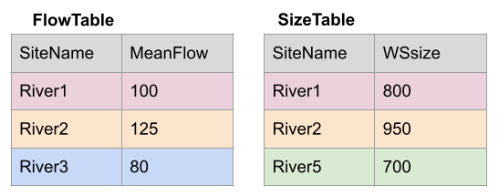
Join setup

Note River1 and River2 match up, but River3 and River5 only exist in one data set or the other.

The first way to deal with this is an INNER JOIN: inner_join() In an inner join, you only keep records that match. So the rows for River3 and River5 will be dropped because there is no corresponding data in the other set. See below:

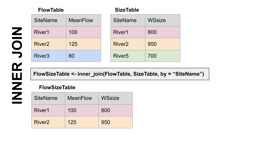
Inner Join

But what if you don’t want to lose the values in one or the other or both?!

For instance, let’s say you have a bunch of discharge data for a stream, and then chemistry grab samples. You want to join the chemistry to the discharge based on the dates and times they were taken. But when you do this, you don’t want to delete all the discharge data where there is no chemistry! We need another option. Enter OUTER JOINS

LEFT JOIN, left_join(): Preserves all values from the LEFT data set, and pastes on the matching ones from the right. This creates NAs where there is a value on the left but not the right. (this is what you’d want to do in the discharge - chemistry example above)

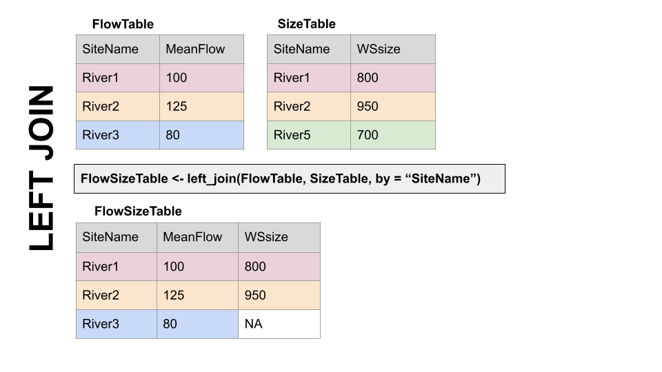
Left Join

RIGHT JOIN, right_join(): Preserves all values from the RIGHT data set, and pastes on the matching ones from the left. This creates NAs where there is a value on the right but not the left.

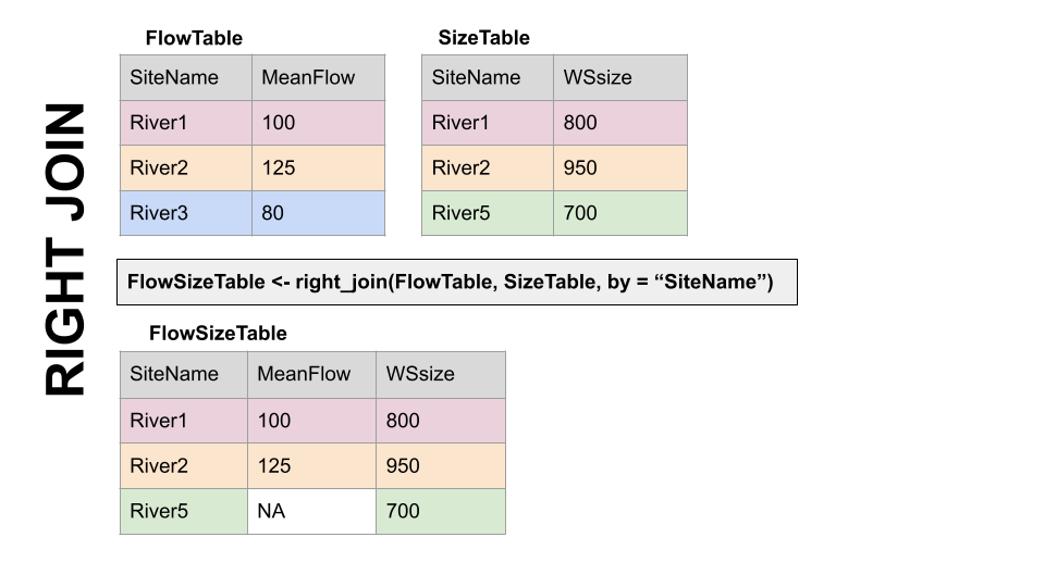
Right Join

FULL JOIN, full_join(): KEEP EVERYTHING! The hoarder of the joins. No matching record on the left? create an NA on the right! No matching value on the right? Create an NA on the left! NAs for everyone!

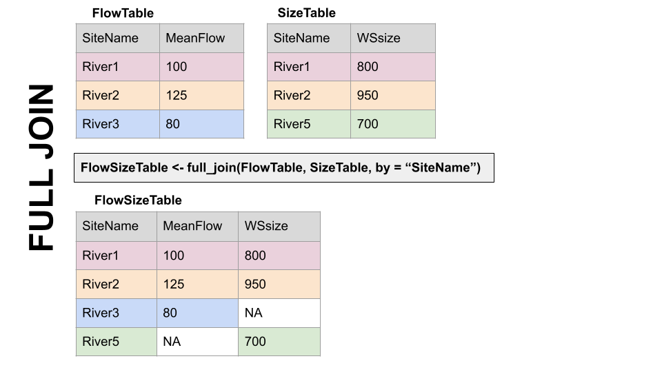
Full Join

When you do this in R, you use the functions identified in the descriptions with the following syntax (see example below):

if the column is named the same in both data sets > xxx_join(left_tibble, right_tibble, by = “key_column”)**

if the column is named differently in both data sets > xxx_join(left_tibble, right_tibble, by = c(“left_key” = “right_key”)

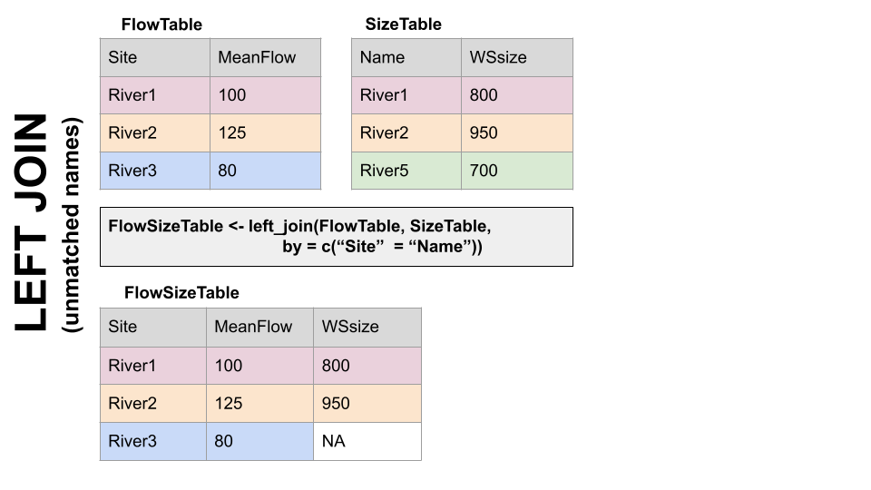
Left Join with differing column names

Note in both of the above, when you specify which column to use as “by” you have to put it in quotes.

Join example¶

So in the chunk below let’s get add the site name by joining the dataAvailable and siteinfo tibbles. They both have the column “monitoring_location_id”, so we can join on that.

What if the same information is in two columns that have different names? Good question! You can do that using the syntax by = c(“left_column” = “right_column”). Clumsy, but we will do an example later.

Finding IDs to download USGS data¶

You can find sites via map and just enter the id like we did in the chunks above: https://maps.waterdata.usgs.gov/mapper/index.html

Below we will look at two other ways to get sites: using a bounding box of a geographic region, or search terms like State.

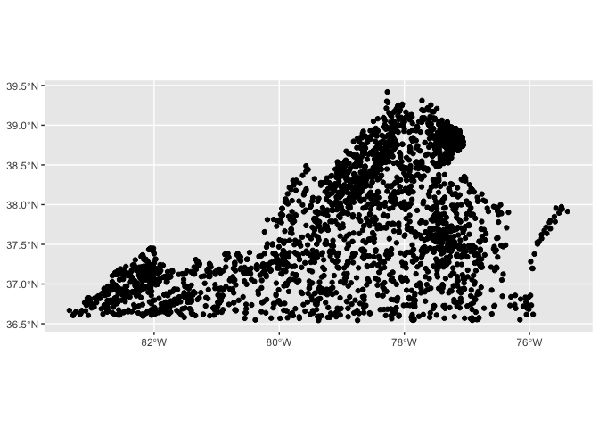
OK let’s download some data!¶

We are going to use read_waterdata_daily(), which downloads daily values.

We will tell it which sites to download, which parameters to download, and then what time period to download.

monitoring_location_id gets the sites we want to download, USGS site numbers, as a character. We will use the swva_sites data we generated (yep, you can download multiple sites at once!)

time gets the start and end dates, together like this: time = c(start, end). IMPORTANT: These must be in YYYY-MM-DD format, but you don’t have to tell R they are dates before you give them to the function, it’ll do that for you.

parameter_code is the parameters you want to download. We want water discharge and water temperature, which are “00060” and “00010”, respectively.

Once the data are downloaded, the temperature and discharge data are stacked on top of each other in the same column (this is LONG data… see later in this chapter). There is a column that tells you what each number is measuring, but it just says the parameter code. To add human-readable information, we can join parameter information in from the parameterCdFile, an object that got added to your environment when you loaded the dataRetrieval package. In Rstudio, if you click the “GlobalEnvironment” dropdown in the “Environment” tab, and then choose dataRetrieval, you can see this object and a couple others.

Let’s plot the water temperature data and discharge as lines and control the color of the lines with the different sites. Because the data is stacked together in one column, we can facet by the column that identifies the measurements (parameter_nm) to make a combined plot of the two.

What could be better about this plot?

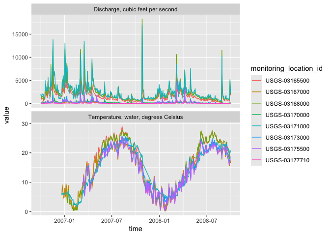
We can add site names with….More joins! Our swva_info data has the names of the sites in human-friendly language. The column in the downloaded data and in the swva_sites data is called “monitoring_location_id” so we just give that to the “by” argument. Perform a left join to add the names of the sites to the data.

Then use select to remove some of the unnecessary columns.

Then make the plot and then snazz it up with labels and a non-junky theme.

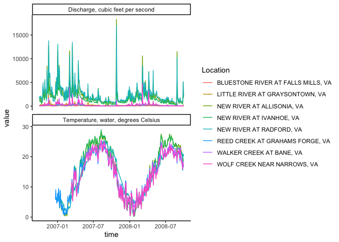
Pivoting: wide and long data¶

Okay, so with the data above: what would you do if you wanted to subtract the discharge or temperature of one gage from another on the same river: to compute rate of change between the two sites, for instance.

You could split them into two objects, then join based on date?

Or…now hear me out… you could PIVOT them.

A two-dimensional object can be either long or wide. Each has its advantages.

LONG

Each observation has its own row. In the first image below, the table on the right is long because each measurement has it’s own row. It’s value and name are identified by other columns, and the values in that column repeat a lot.

WIDE

Observations of different things have their own columns. In the first image below, notice in the left hand table there are “Flow”, “Temp”, and “NO3” columns rather than an identifier in a separate column like in the table on the right.

Why?

Long and wide data are more efficient for different things. Think about plotting a data set with 10 stream gages. If they are in a long format, you can just add color = Gage to your ggplot aes(). If they are in a wide format, meaning each gage has it’s own column, you’d have to write a new geom for EACH gage, because they’re all in separate columns.

Now imagine you want to do some math to create new data: let’s say NO3 multiplied by Flow…. How would you even do that using the data on the right? With the wide data on the left it is simply mutate(NO3 * Flow).

Finally, which table is easier to read in TABLE format (not a plot) in each of the two images below? Wide data is much more fitting for tables.

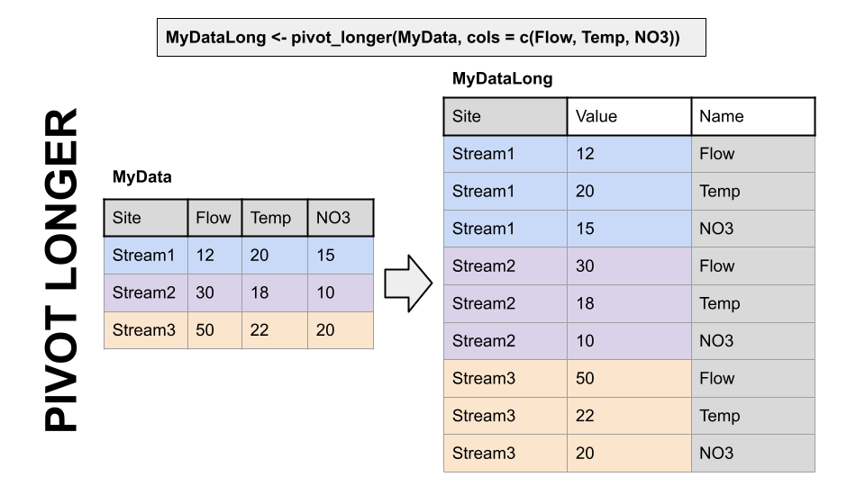
Pivoting to a longer format

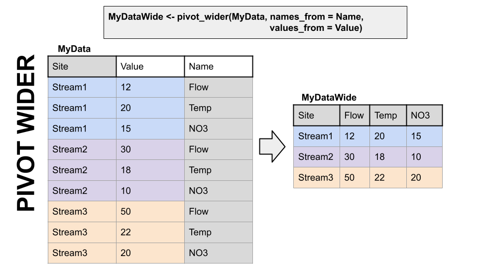
Pivoting to a wider format

dplyr, part of the tidyverse, has functions to convert data between wide and long data. I have to look up the syntax every single time I use them. But they are VERY useful.

Pivot Examples¶

Back to our original question: I want to subtract the flow at Ivanhoe from the flow at Radford on the new river to see how much flow increases between the two sites through time.

To do this I am going to use pivot_wider() to give Ivanhoe and Radford discharges their own column.

First, we will trim to just discharge data using a filter, then use select to trim the data to just the columns we need, then call pivot_wider telling it which data to use for the new column names (names_from = monitoring_location_name) and what values we want to pivot into the data under those columns (values_from = value).

Then, subtract the two and make a plot!

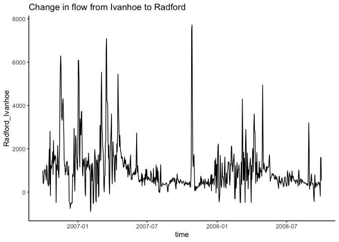
To further illustrate how to move between long and wide data and when to use them, let’s grab some water quality data. This process will also review some of the other concepts from this topic.

In the chunk below we will find sites from our SWVA bounding box that are on the New River and then download any data they have for chloride and specific conductance.

We will use readWQPqw() to read the chemistry data.

Now, let’s clean things up a bit. Hang on tight, we are going to do a bunch of data wrangling in one pipe sequence to accomplish what we want: A dataset that has chloride and specific conductance in their own columns, with a column for time, and one that says what site the measurement was from.

This will allow us to plot Chloride vs. specific conductance

The workflow is as follows: - Create a time column that combines the date and time columns in the downloaded data. - Select the columns we need to pivot the data wider - Pivot wider - Rename the specific conductance column so it doesn’t have a space in it - Join in the names of the locations - Select just the columns we want

Finally plot chloride on the x axis, specific conductance on the y, and color by site!

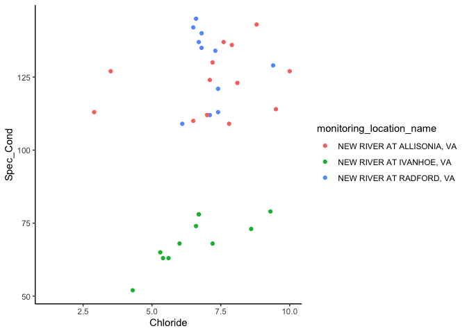
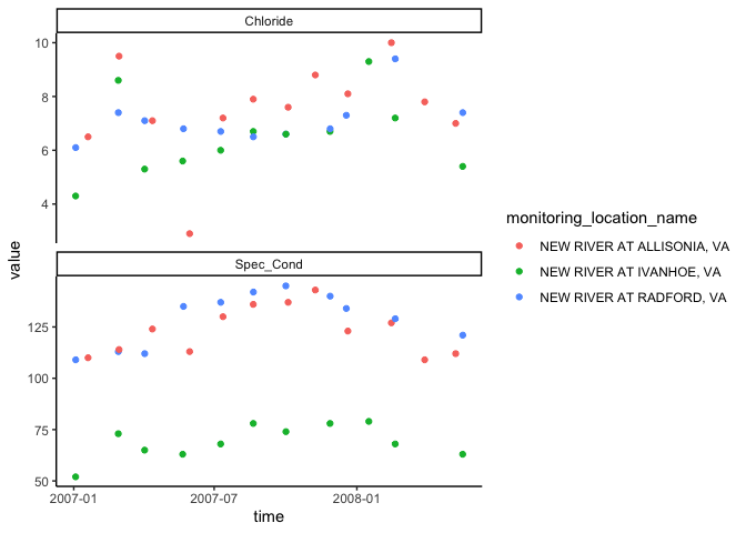
Finally, let’s look at how to pivot the same dataset longer. An example of why you might want to do this is if you want to make a stacked plot with Chloride on one and specific conductance on the other, both against time, using the ggplot facets, not making multiple plots.

So! We will pivot longer, telling pivot_longer() to pivot the column Spec_Cond and Chloride.

When we plot this, we will see that there is one datapoint from way before all the others, so we will filter that out so we can see the pattern in the rest of the data.